Volume 27, Number 3—March 2021
Research
Daily Forecasting of Regional Epidemics of Coronavirus Disease with Bayesian Uncertainty Quantification, United States
Cite This Article
Citation for Media
Abstract
To increase situational awareness and support evidence-based policymaking, we formulated a mathematical model for coronavirus disease transmission within a regional population. This compartmental model accounts for quarantine, self-isolation, social distancing, a nonexponentially distributed incubation period, asymptomatic persons, and mild and severe forms of symptomatic disease. We used Bayesian inference to calibrate region-specific models for consistency with daily reports of confirmed cases in the 15 most populous metropolitan statistical areas in the United States. We also quantified uncertainty in parameter estimates and forecasts. This online learning approach enables early identification of new trends despite considerable variability in case reporting.
Coronavirus disease (COVID-19), caused by severe acute respiratory syndrome coronavirus 2 (SARS-CoV-2) (1), was detected in the United States in January 2020 (2). Researchers documented deaths in the United States caused by COVID-19 in February (3). Thereafter, surveillance testing expanded nationwide (4). These and other efforts revealed community spread across the United States and exponential growth of new COVID-19 cases throughout most of March. Growth of cases during February–April had a doubling time of 2–3 days (5), similar to the doubling time of the initial outbreak in China (6). The rapid increase in cases prompted broad adoption of social distancing practices such as teleworking, travel restrictions, use of face masks, and government mandates prohibiting public gatherings (7). The United States soon became a hotspot of the COVID-19 pandemic. In the United States, detection of new cases peaked in late April and steadily declined until mid-June (4). The decline in case numbers suggest that mandates and social distancing interventions effectively slowed COVID-19 transmission. Efforts to quantify the effects of these measures indicate that they substantially reduced disease prevalence (8,9).
In mid-June and mid-September 2020, the daily incidence of COVID-19 cases in the United States increased a second and third time (4). Public health officials must effectively monitor ongoing COVID-19 transmission to quickly respond to dangerous upticks in disease. To contribute to situational awareness of COVID-19 transmission dynamics, we developed a mathematical model for the daily incidence of COVID-19 in each of the 15 most populous US metropolitan statistical areas (MSAs) (10). Each model is composed of ordinary differential equations (ODEs) characterizing the dynamics of various populations, including subpopulations that did or did not practice social distancing.
We used online learning to calibrate our models for consistency with historical case reports. We also applied Bayesian methods to quantify uncertainties in predicted detection of new cases. This approach enabled identification of new epidemic trends despite variability in case detection. These findings can inform policymakers designing evidence-based responses to regional COVID-19 epidemics in the United States.
Data Used in Online Learning
We obtained reports of new confirmed cases from the GitHub repository maintained by The New York Times newspaper (11). Each day, at varying times of day, we updated the model using cumulative data since January 21, 2020. The data in this analysis is from January 21–June 26, 2020. We aggregated county-level data to obtain case counts for each of the 15 most populous US MSAs, which encompass the following cities: New York City, New York; Los Angeles, California; Chicago, Illinois; Dallas, Texas; Houston, Texas; Washington, DC; Miami, Florida; Philadelphia, Pennsylvania; Atlanta, Georgia; Phoenix, Arizona; Boston, Massachusetts; San Francisco, California; Riverside, California; Detroit, Michigan; and Seattle, Washington.
The political entities comprising each MSA are those delineated by the federal government (10). The number of political units (i.e., counties and independent cities) in the MSAs of interest ranged from 2 (for the Los Angeles and Riverside MSAs) to 29 (for the Atlanta MSA). The median number of counties in an MSA was 7; the mean was 10. The number of states encompassing an MSA ranged from 1 (for 8/15 MSAs) to 4 (for Philadelphia). The median number of encompassing states was 1; the mean was 2.
COVID-19 Transmission Model and Parameters
We used daily reports of new cases to parameterize a compartmental model for the regional COVID-19 epidemic in each of the 15 MSAs of interest. Until June 2020, we also parameterized curve-fitting models. However, curve-fitting models can generate only single-peak epidemic curves, so we abandoned this approach after the MSAs of interest all experienced multiple waves of disease (Appendix 1).
Figure 1
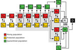
Figure 1. Illustration of the populations and processes considered in a mechanistic compartmental model of coronavirus disease daily incidence during regional epidemics, United States, 2020. The model accounts for susceptible persons (...
Each MSA-specific model accounted for 25 populations (Figure 1; Appendix 1 Figure 1). We considered infectious persons to be exposed and incubating virus (i.e., presymptomatic), asymptomatic while clearing virus, or symptomatic. The parameter ρE characterized the relative infectiousness of exposed persons and ρA characterized that of asymptomatic persons compared with symptomatic persons. In our model, infected persons quarantined with rate constant kQ and symptomatic persons with mild disease quarantined with rate constant jQ. We modeled social distancing by enabling the movement of susceptible and infectious persons between mixing and socially distanced (i.e., protected) populations. The size of the protected population was determined by 2 parameters: λi, a rate constant; and pi, a steady-state population setpoint, where index i refers to the current social distancing period. The model accounts for varying adherence to social distancing practices over time by using n distinct social distancing periods after an initial period of social distancing. Persons in the protected population were less likely to be infected and less likely to transmit disease by a factor mb. Within the mixing population, disease was transmitted with rate constant β. The model reproduced a nonexponentially distributed incubation period by dividing the incubation period into 5 sequential stages of equal mean duration, given by 1/kL. We considered infected persons in the first stage of the incubation period to be noninfectious and undetectable. A fraction of exposed persons, fA, left the incubation period without symptoms. The remaining persons left with symptoms. The other symptomatic persons, fH, progressed to severe disease; the remainder had mild disease and recovered. The fraction of persons with severe disease who recovered is denoted as fR; the others died. We considered hospitalized persons (or those at home with severe disease) to be quarantined. Persons left the asymptomatic state with rate constant cA, left the mild disease state with rate constant cI, and left the severe disease/hospitalized state with rate constant cH.
The model consisted of 25 ODEs (Appendix 1 Equations 1–17). Each state variable of the model represented the size of a population. In addition to the 25 ODEs, we considered an auxiliary 1-parameter measurement model that related state variables to expected case reporting (Appendix 1 Equations 23, 24) and a negative binomial model for variability in new case detection (Appendix 1 Equations 25–27). We designed the model to consider multiple periods of social distancing with distinct setpoints for the quasistationary protected population size. The model always included an initial period of social distancing. The number of additional social distancing periods was given by n. Here, we considered only 2 cases: n = 0 and n = 1. We determined the best value of n by using model selection (Appendix 1).
The compartmental model and the auxiliary measurement model for n = 0 had a total of 20 parameters. We considered 6 of these parameters to have adjustable values (Table 1) and 14 to have fixed values (Tables 2, 3) (12–20; Appendix 1). The adjustable model parameters were t0, the start time of the local epidemic; σ>t0, the time at which the initial social distancing period began; p0, the quasistationary fraction of the total population practicing social distancing; λ0, an eigenvalue characterizing the rate of movement between the mixing and protected subpopulations and establishing a timescale for population-level adoption of social distancing practices; and β, which characterized the rate of disease transmission in the absence of social distancing. The measurement model parameter fD represented the time-averaged fraction of new cases detected. Inference of adjustable parameter values was based on a negative binomial likelihood function (Appendix 1 Equation 27). The dispersal parameter r of the likelihood was adjustable; its value was jointly inferred with those of t0, σ, p0, λ0, β, and fD.
The compartmental model had 3 adjustable parameters for each additional social distancing period after the initial. For 1 additional period of social distancing (n = 1, the additional adjustable parameters were τ1>σ, the onset time of second-phase social distancing; p1, the second-phase quasistationary setpoint; and λ1, which determined the timescale for transition from first- to second-phase social distancing behavior. For a second social distancing period, we replaced p0 with p1 and λ0 with λ1 at time t = τ1. If adherence to effective social distancing practices began to relax at time t = τ1, then p1<p0.
Statistical Model for Noisy Case Reporting
We used a deterministic compartmental model to predict the expected number of new confirmed COVID-19 cases reported daily. In other words, we assumed that the number of new cases reported over a 1-day period was a random variable and that the expected value would follow a deterministic trajectory. We further assumed that day-to-day fluctuations in the random variable were independent and characterized by a negative binomial distribution, denoted as NB(r,p). We used NB(r,p) to model noise in reporting and case detection. The support of this distribution is the nonnegative integers, which is natural for populations. Furthermore, the shape of NB(r,p) is flexible enough to recapitulate an array of unimodal empirical distributions. With these assumptions, we obtained a likelihood function (Appendix 1 Equation 27) in the form of a product of probability mass functions of NB(r,p). Formulation of a likelihood is a prerequisite for standard Bayesian inference; however, some related methods, such as approximate Bayesian computation, do not rely on a likelihood function.
Online Learning of Model Parameter Values through Bayesian Inference
We used Bayesian inference to identify adjustable model parameter values for each MSA of interest. In each inference, we assumed a uniform prior and used an adaptive Markov chain Monte Carlo algorithm (21) to generate samples of the posterior distribution for the adjustable parameters (Appendix 1).
The maximum a posteriori (MAP) estimate of a parameter is the value corresponding to the mode of its marginal posterior, where probability mass is highest. Because we assumed a uniform prior, our MAP estimates were maximum-likelihood estimates.
Forecasting with Quantification of Prediction Uncertainty: Bayesian Predictive Inference
In addition to inferring parameter values, we quantified uncertainty in predicted trajectories of daily case reports. We obtained a predictive inference of the expected number of new cases detected on a given day by parameterizing a model using a randomly-chosen parameter posterior sample generated in Markov chain Monte Carlo sampling. We then predicted the number of cases detected by adding a noise term, drawn from NB(r,p), where r is set at the randomly sampled value and p is set using an equation (Appendix 1 Equation 26).
We used LSODA (22; SciPy, https://scipy.org) to numerically integrate the described ODEs and obtain a prediction of the compartmental model for any given (1-day) surveillance period and specified settings for parameter values (Appendix 1 Equations 1–17, 23). The initial condition was defined by the inferred value of t0 (Table 1) and the fixed settings for S0 and I0 (Tables 2, 3). We predicted the actual number of new cases detected by entering the predicted expected number of new cases into an equation (Appendix 1 Equation 29).
The 95% credible interval (CrI) for the predicted number of new case reports on a given day is the central part of the marginal predictive posterior capturing 95% of the probability mass. This region is bounded above by the 97.5th percentile and below by the 2.5th percentile.
The objective of our study was to detect notable new trends in daily COVID-19 incidence as early as possible. We achieved this goal by systematically and regularly updating mathematical models capturing historical trends in regional COVID-19 epidemics using Bayesian inference and making forecasts with Bayesian uncertainty quantification.
Figure 2
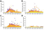
Figure 2. Temporal correlations of fractional case counts of coronavirus disease in and around the New York City, New York, metropolitan statistical area, United States, March 1–June 13, 2020. The fractional case...
Our analysis focused on the populations of US cities and their MSAs instead of regional populations within other political boundaries, such as those of US states. The boundaries of MSAs are based on social and economic interactions (10), which suggests that the population of an MSA is likely to be more uniformly affected by the COVID-19 pandemic than, for example, the population of a state. Accordingly, daily reports of new COVID-19 cases for the New York City MSA (Figure 2, panel A) are more temporally correlated than for the 3 states that make up the New York City MSA: New York (Figure 2, panel B), New Jersey (Figure 2, panel C), and Pennsylvania (Figure 2, panel D). Daily case counts for New Jersey resembled those for New York City because the 2 populations overlap considerably: ≈74% of New Jersey’s population is part of the New York City MSA and ≈32% of the population of the New York City MSA is part of New Jersey (13).
Figure 3
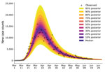
Figure 3. Illustration of Bayesian predictive inference for daily new case counts of coronavirus disease in the New York City, New York, metropolitan statistical area, United States, March 1–June 21, 2020. Daily...
For each of the 15 most populous US MSAs, we defined parameters for a compartmental model using MSA-specific surveillance data, namely aggregated county-level reports indicating the number of new confirmed COVID-19 cases within a given MSA each day. We made daily predictions by using Bayesian parameterization and forecasting with uncertainty quantification (UQ) for each of the 15 MSAs (Figure 3). Predictions took the form of a predictive posterior distribution and varied because of the uncertainties in adjustable model parameter estimates, which were characterized quantitatively through Bayesian inference. For these inferences we used the complete time series of available daily new case counts for the region of interest.
Figure 4
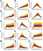
Figure 4. Bayesian predictive inferences for daily new case counts of coronavirus disease in the 15 most populous metropolitan statistical areas, United States, March 1–June 21, 2020. Predictions conditioned on the compartmental...
We conducted predictive inferences for all 15 MSAs of interest (Figure 4). We conditioned our predictions on the compartmental model with n = 0. These results demonstrate that, for the timeframe of interest, the compartmental model with n = 0 can reproduce many of the empirical epidemic curves for the MSAs of interest, which vary in shape.
Figure 5
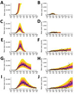
Figure 5. Illustration of the need for online learning for modeling daily new case counts of coronavirus disease in the New York City, New York, and Phoenix, Arizona, metropolitan statistical areas, United...
We also calculated predictive inferences for the New York City and Phoenix MSAs over time (Figure 5; Appendix 2 Videos 1, 2). These results illustrate that accurate short-term predictions are possible; however, continual updating of parameter estimates is required to maintain accuracy.
Figure 6
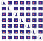
Figure 6. Matrix of 1- and 2-dimensional projections of the 7-dimensional posterior samples obtained for the adjustable parameters associated with the compartmental model (n= 0) for daily new case counts...
We found that the adjustable parameters of the compartmental model had identifiable values, meaning that their marginal posteriors were unimodal (Figure 6). In the context of a deterministic model, the significance of identifiability is that, despite uncertainties in parameter estimates, we can expect predictive inferences of daily new case reports to cluster around a central trajectory. The results are representative (Figure 6); we routinely recovered unimodal marginal posteriors. However, we do not have a mathematical proof of identifiability for our model.
Usually, when we forecasted with UQ, the empirical new case count for the day immediately following our inference (+1), and often for each of several additional days, fell within the 95% CrI of the predictive posterior. When the reported number of new cases falls outside the 95% CrI and above the 97.5 percentile, we interpret this upward-trending rare event to have a probability of <0.025, assuming the model is both explanatory (i.e., consistent with historical data) and predictive of the near future. If the model is predictive of the near future, the probability of 2 consecutive rare events is far smaller, <0.001. Thus, consecutive upward-trending rare events, called upward-trending anomalies, can indicate that the model is not predictive. An anomaly suggests that the rate of COVID-19 transmission has increased beyond what can be explained by the model.
Figure 7
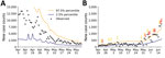
Figure 7. Rare events and anomalies in daily new case counts of coronavirus disease in (A) the New York City, New York metropolitan statistical area during April 5–June 4, 2020 and (B)...
We did not observe upward-trending anomalies for the New York City MSA (Figure 7, panel A). However, for the Phoenix MSA, we observed several anomalies that preceded rapid and sustained growth in the number of new cases reported per day in June (Figure 7, panel B).
Figure 8
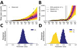
Figure 8. Predictions of the compartmental model for daily new case counts of coronavirus disease in the Phoenix, Arizona, metropolitan statistical area, United States, January 21–June 18, 2020. A) Model using 1...
We assumed these anomalies arose from behavioral changes. To explain them, we enabled the compartmental model to account for a second social distancing period by increasing the setting for n from 0 to 1. With this change, the number of adjustable parameters increased from 7 to 10. One of the new parameters was τ1, the start time of the second social distancing period. The other new parameters, λ1 and p1, replaced λ0 and p0 at time t = τ1 The compartmental model with 2 social distancing periods better explained the data from Phoenix than the compartmental model with only 1 social distancing period (Figure 8, panels A and B). This conclusion is supported by the Akaike and Bayesian information criteria values for the 2 scenarios (Appendix 1 Table 1). Although these criteria are crude model selection tools in the context of non-Gaussian posteriors, we decided that they were adequately discriminatory. Each strongly indicates that the model with 2 social distancing periods better represented the data than the model with 1 social distancing period. Furthermore, the MAP estimate for p1 (≈0.38) was less than that for p0 (≈0.49) (Figure 8, panels C, D) and the marginal posteriors for these parameters were largely nonoverlapping (Figure 8, panel D). These findings suggest that the increase in COVID-19 cases in Phoenix can be explained by relaxation in social distancing practices, quantified by our estimates for p0 and p1. The MAP estimate of the start time of the second period of social distancing corresponds to May 24, 2020 (95% CrI May 20–28, 2020). Overall, 8 of the 9 observed anomalies occurred after this period, the first of which occurred on June 2, 2020 (Figure 8, panel B).
We hypothesized that a single event generating thousands of new infections, such as a mass gathering, might prompt a new upward trend in COVID-19 transmission. However, simulations for New York City and Phoenix did not support this hypothesis (Appendix 1 Figure 2). In each of these simulations, we moved a specified number of persons from the mixing susceptible population SM into the exposed population E1 at the indicated time, May 30, 2020. Each perturbation increased disease incidence but had minimal effect on the slope of the trajectory of new case detection.
In addition to Phoenix, 4 other MSAs had contemporaneous trends explainable by relaxation of social distancing (Appendix 1 Table 1, Figure 3). MAP estimates for τ1 indicate that the second social distancing period began on May 27, 2020 in Houston; April 19, 2020 in Miami; May 24, 2020 in Phoenix; June 12, 2020 in San Francisco; and June 7, 2020 in Seattle (Appendix 1 Figure 3). We detected upward-trending anomalies for these 5 MSAs (Appendix 1 Figure 4, panels A–D), but not for 3 of 4 other MSAs that had epidemic curves consistent with sustained social distancing (Appendix 1 Figure 4, panels E–H; Appendix 2 Videos 3–10). We assessed the overall prediction accuracy of the region-specific compartmental models (Appendix 1 Figure 5).
We found that online learning of model parameter values from real-time surveillance data is feasible for mathematical models of COVID-19 transmission. Furthermore, we found that predictive inference of the daily number of new cases reported is feasible for regional COVID-19 epidemics occurring in multiple US MSAs. We are continuing to perform daily forecasts and to disseminate the results (23,24). Inferences are computationally expensive and the cost increases as new data become available; thus, daily inferences using these methods might be impractical in some circumstances.
These predictive inferences can be used to identify harbingers of future growth in COVID-19 transmission rates. We found that 2 consecutive upward-trending rare events in which the number of new cases reported is above the upper limit of the 95% CrI of the predictive posterior might indicate potential for increased transmission during the following days to weeks. This feature might be especially predictive when anomalies are accompanied by increasing prediction uncertainty, as seen in Phoenix (Figure 7, panel B).
We found that the June increase in transmission rate of COVID-19 in the Phoenix metropolitan area can be explained by a reduction in the percentage of the population adhering to effective social distancing practices from ≈49% to ≈38% (Figure 8, panel D). However, our study sheds no light on which social distancing practices are effective at slowing COVID-19 transmission. We inferred that relaxation of social distancing measures began around May 24, 2020 (Figure 8, panel B). Contemporaneous upward trends in the rate of COVID-19 transmission in the Houston, Miami, San Francisco, and Seattle MSAs can also be explained by relaxation of social distancing (Appendix 1 Table 1, Figure 3). These findings are qualitatively consistent with earlier studies indicating that social distancing is effective at slowing the transmission of COVID-19 (7,8). These results also suggest that the future course of the pandemic is controllable, especially with accurate recognition of when stronger nonpharmaceutical interventions are needed to slow COVID-19 transmission.
One limitation of our study is that trend detection is data-driven, which means that a new trend cannot be detected until enough evidence has accumulated. Our analysis used reports of new cases, which reflect transmission dynamics of the past days to weeks rather than the current moment. Other types of surveillance data, such as assays of viral RNA in wastewater samples, also might improve situational awareness. Another limitation is that our inferences are based on a mathematical model associated with considerable structure and fixed parameter uncertainties and simplifications. Among the simplifications is the replacement of certain time-varying parameters, such as those characterizing testing capacities, with constants, which are assumed to provide an adequate time-averaged characterization. In this study, we used a deterministic compartmental model. If disease prevalence decreases, a stochastic version of the model might be more appropriate for forecasting efforts. Although the model can reproduce historical data and make accurate short-term forecasts, its structure and fixed parameters are subject to revision as we learn more about COVID-19. Furthermore, the model will need to be revised to account for vaccination. Results from serologic studies and estimates of excess deaths should enable model improvements.
Dr. Lin is a scientist in the Information Sciences Group of the Computer, Computational, and Statistical Sciences Division at Los Alamos National Laboratory. His primary research interest is the development and application of advanced data science methods in the modeling of biological systems.
Acknowledgments
This article was preprinted at https://arxiv.org/abs/2007.12523.
Y.T.L. received financial support from the Laboratory Directed Research and Development Program at Los Alamos National Laboratory (Project XX01); this support enabled early feasibility studies. Y.T.L., C.S., J.R., G.T., S.C., and W.S.H. were supported by the US Department of Energy Office of Science through the National Virtual Biotechnology Laboratory, a consortium of national laboratories (Argonne, Los Alamos, Oak Ridge, and Sandia) focused on responding to COVID-19, with funding provided by the Coronavirus CARES Act. J.N., E.M., and R.G.P. were supported by the National Institute of General Medical Sciences of the National Institutes of Health (grant no. R01GM111510). A.M. received financial support from the 2020 Mathematical Sciences Graduate Internship program, which is sponsored by the Division of Mathematical Sciences of the National Science Foundation. Computational resources were from the Darwin cluster at Los Alamos National Laboratory, which is supported by the Computational Systems and Software Environment subprogram of the Advanced Simulation and Computing program at Los Alamos National Laboratory, which is funded by National Nuclear Security Administration of the US Department of Energy. Computational resources also came from Northern Arizona University’s Monsoon computer cluster, which is funded by Arizona’s Technology and Research Initiative Fund.
References
- Gorbalenya AE, Baker SC, Baric RS, de Groot RJ, Drostetn C, Gulyaeva AA, et al.; Coronaviridae Study Group of the International Committee on Taxonomy of Viruses. The species Severe acute respiratory syndrome-related coronavirus: classifying 2019-nCoV and naming it SARS-CoV-2. Nat Microbiol. 2020;5:536–44. DOIPubMedGoogle Scholar
- Ghinai I, McPherson TD, Hunter JC, Kirking HL, Christiansen D, Joshi K, et al.; Illinois COVID-19 Investigation Team. First known person-to-person transmission of severe acute respiratory syndrome coronavirus 2 (SARS-CoV-2) in the USA. Lancet. 2020;395:1137–44. DOIPubMedGoogle Scholar
- Holshue ML, DeBolt C, Lindquist S, Lofy KH, Wiesman J, Bruce H, et al.; Washington State 2019-nCoV Case Investigation Team. First case of 2019 novel coronavirus in the United States. N Engl J Med. 2020;382:929–36. DOIPubMedGoogle Scholar
- The Atlantic Monthly Group. The COVID Tracking Project. 2020 [cited 2020 Jul 1]. https://covidtracking.com/data/national
- Silverman JD, Hupert N, Washburne AD. Using influenza surveillance networks to estimate state-specific prevalence of SARS-CoV-2 in the United States. Sci Transl Med. 2020;12:
eabc1126 . DOIPubMedGoogle Scholar - Sanche S, Lin YT, Xu C, Romero-Severson E, Hengartner N, Ke R. High contagiousness and rapid spread of severe acute respiratory syndrome coronavirus 2. Emerg Infect Dis. 2020;26:1470–7. DOIPubMedGoogle Scholar
- Coronavirus Resource Center, Johns Hopkins University. Timeline of COVID-19 policies, cases, and deaths in your state: a look at how social distancing measures may have influenced trends in COVID-19 cases and deaths. 2020 [2020 Jul 1]. https://coronavirus.jhu.edu/data/state-timeline
- Courtemanche C, Garuccio J, Le A, Pinkston J, Yelowitz A. Strong social distancing measures in the United States reduced the COVID-19 growth rate. Health Aff (Millwood). 2020;39:1237–46. DOIPubMedGoogle Scholar
- Hsiang S, Allen D, Annan-Phan S, Bell K, Bolliger I, Chong T, et al. The effect of large-scale anti-contagion policies on the COVID-19 pandemic. Nature. 2020;584:262–7. DOIPubMedGoogle Scholar
- Executive Office of the President. OMB bulletin no. 15-01. 2020 [cited 2020 Jul 1]. https://www.bls.gov/bls/omb-bulletin-15-01-revised-delineations-of-metropolitan-statistical-areas.pdf
- The New York Times. Coronavirus (Covid-19) data in the United States. 2020 [cited 2020 Jul 1]. https://github.com/nytimes/covid-19-data
- Lauer SA, Grantz KH, Bi Q, Jones FK, Zheng Q, Meredith HR, et al. The incubation period of coronavirus disease 2019 (COVID-19) from publicly reported confirmed cases: estimation and application. Ann Intern Med. 2020;172:577–82. DOIPubMedGoogle Scholar
- United States Census Bureau. Metropolitan and micropolitan statistical areas population totals and components of change: 2010–2019. 2020 [cited 2020 Jul 1]. https://www.census.gov/data/tables/time-series/demo/popest/2010s-total-metro-and-micro-statistical-areas.html
- Arons MM, Hatfield KM, Reddy SC, Kimball A, James A, Jacobs JR, et al.; Public Health–Seattle and King County; CDC COVID-19 Investigation Team. Presymptomatic SARS-CoV-2 infections and transmission in a skilled nursing facility. N Engl J Med. 2020;382:2081–90. DOIPubMedGoogle Scholar
- Nguyen VVC, Vo TL, Nguyen TD, Lam MY, Ngo NQM, Le MH, et al. The natural history and transmission potential of asymptomatic SARS-CoV-2 infection. Clin Infect Dis 2020 Jun 4 [Epub ahead of print].
- Ministry of Health, Labour and Welfare of Japan. Official report on the cruise ship Diamond Princess, May 1, 2020. 2020 [cited 2020 Jul 1]. https://www.mhlw.go.jp/stf/newpage_11146.html
- Sakurai A, Sasaki T, Kato S, Hayashi M, Tsuzuki SI, Ishihara T, et al. Natural history of asymptomatic SARS-CoV-2 infection. N Engl J Med. 2020;383:885–6. DOIPubMedGoogle Scholar
- Perez-Saez J, Lauer SA, Kaiser L, Regard S, Delaporte E, Guessous I, et al. Serology-informed estimates of SARS-COV-2 infection fatality risk in Geneva, Switzerland. Lancet Infect Dis. 2020 Jul 14 [Epub ahead of print]. https://doi.org/10.1016/S1473-3099(20)30584-3
- Richardson S, Hirsch JS, Narasimhan M, Crawford JM, McGinn T, Davidson KW, et al.; the Northwell COVID-19 Research Consortium. Presenting characteristics, comorbidities, and outcomes among 5700 patients hospitalized with COVID-19 in the New York City area. JAMA. 2020;323:2052–9. DOIPubMedGoogle Scholar
- Wölfel R, Corman VM, Guggemos W, Seilmaier M, Zange S, Müller MA, et al. Virological assessment of hospitalized patients with COVID-2019. Nature. 2020;581:465–9. DOIPubMedGoogle Scholar
- Hindmarsh AC. ODEPACK, a systematized collection of ODE solvers. In: Stepleman RS, editor. Scientific computing: applications of mathematics and computing to the physical sciences. Amsterdam: North-Holland Publishing Company; 1983. p. 55–64.
- U.S. Department of Energy. COVID-19 pandemic modeling and analysis. 2020 [cited 2020 Jul 1]. https://covid19.ornl.gov
- Lin YT, Neumann J, Miller EF, Posner RG, Mallela A, Safta C, et al. Los Alamos COVID-19 city predictions. 2020 [cited 2020 Jul 1]. https://github.com/lanl/COVID-19-Predictions.
Figures
Tables
Cite This ArticleOriginal Publication Date: February 10, 2021
Table of Contents – Volume 27, Number 3—March 2021
| EID Search Options |
|---|
|
|
|
|
|
|
Please use the form below to submit correspondence to the authors or contact them at the following address:
Yen Ting Lin, CCS-3, Los Alamos National Laboratory, Mailstop B256, 1 Bikini Atoll, Los Alamos, NM 87545, USA
Top